This post is based on the 732A92 Texting Mining course, given by Marco Kuhlmann at LiU in 2019.

---

Word embeddings

對於人來說，要理解文字並不是件困難的事，但對電腦來說，每個字不過是一串 string，所以當我們要做 text mining 時就必須要將這些 string 轉化成電腦可以理解的方式。 而 word embedding(word vector or word representation) 的概念就是將文字轉換成 vector ，好讓電腦可以讀懂文字間的關係。

譬如說，人類可以理解 pretty 和 beautiful 是相近詞，但如果只是給電腦這兩個單字，對於電腦來說，這只是兩個不同長度的 string 罷了。word embedding 會將這兩個字轉換成不同的 vector 映射到一個高維空間，當這兩個 vector 越接近（可以使用 consine similarity）就表示這兩個詞越相近。這就是 word embedding 主要的概念。

• A word embedding is a mapping of words to points in a vector space such that nearby words (points) are similar in terms of their distributional properties.

The distributional principle

word embedding 方法可以使用最重要的就是因為有 distributional hypothesis 這個假設。

• The distributional principle states that words that occur in similar contexts tend to have similar meanings.

這裡的概念是說，詞(target words)出現在類似的上下文中(context words)，則它們很有可能有相似的意思。 譬如說，
-「那隻『貓』好可愛」
-「那隻『狗』好可愛」
這時候除了『貓』和『狗』外，這兩句話的上下文是一樣的，根據 distributional principle，這兩個詞應該是相似的。

Co-occurrence matrix

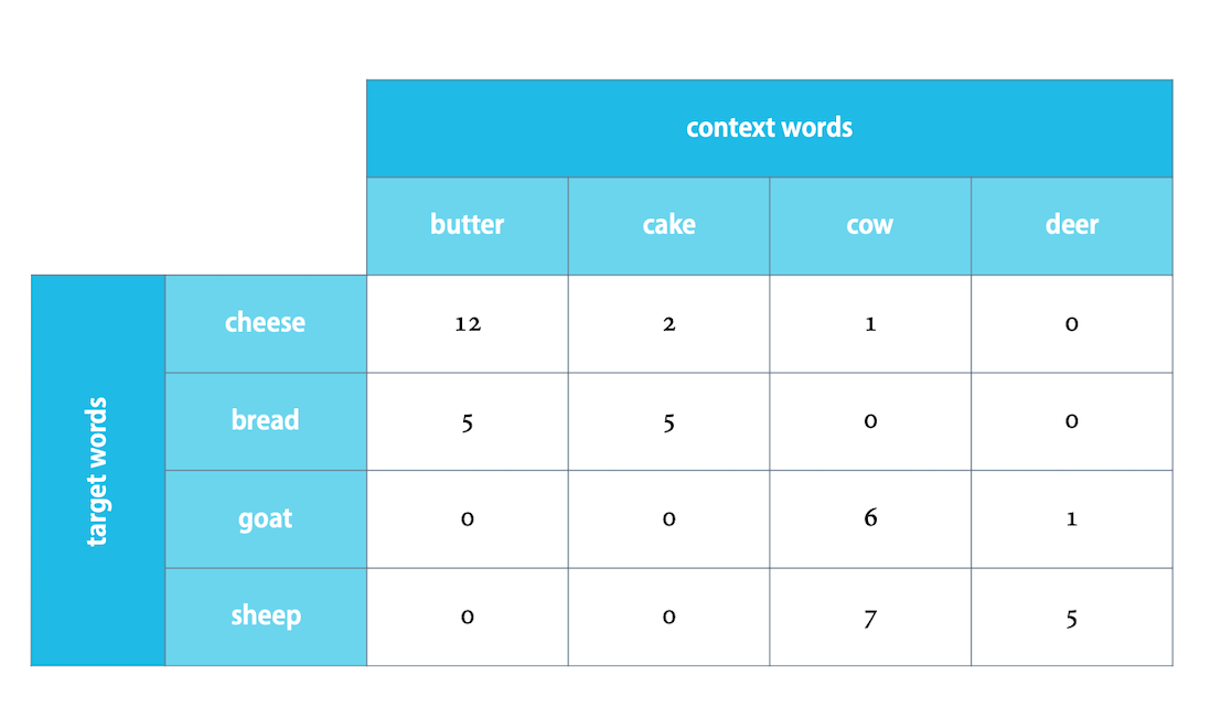
上圖中，context words 就是上下文，而 target words 就是我們想要分析的字詞。
現在來看 cheese 這個字，可以看到和 butter, cake, cow, deer 這幾個字一起出現的次數分別是，12, 2, 1和0次。看起來和 butter 還有 cake 連結性比較強。 再來看 bread 這個字，同樣的在 butter 和 cake 上的連結也比較強。如果我們把這兩個單字用向量表示就會是，(12, 2, 1, 0) 和 (5, 5, 0, 0)，可以去比較和其他兩個單字的 cosine similarity，這兩個的關係是比較強的。

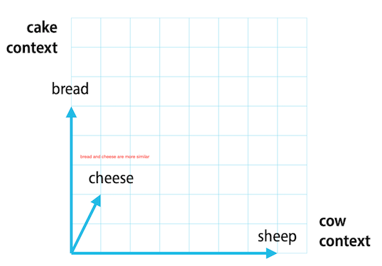
現在我們把它們畫出來（因為它們被映射到的是四維空間，所以老師的 slide 只看 cow 和 cake 這兩個 context words）

如果還是不太明白，這篇部落格應該可以看懂。

補充： 從上面的 matrix 可能會想到一件事，context words 等於是決定了 target words 的向量啊！ 換句話說，當我們分析不同的文本的時候，會需要不同的 context words來算出 word embeddings。想像，如果今天要分析新聞報導和 ptt 內容，不太可能使用一樣的 context words，畢竟ptt用語和新聞用語會有很大的不同。（蛤？你說記者都抄 ptt 內容嗎？XDDD）

---

Simple applications of word embeddings

word embeddings 的應用

• finding similar words. 找到相似的字，像是上面的例子，找出哪一個字和 cheese 比較相似。
• answering ‘odd one out’ questions. 找出不一樣的詞，譬如說 lunch, breakfast, dinner, car 哪一個詞屬於不同類？ (根據上面提到的概念，lunch, breakfast, dinner 這三個的 vector 應該會比較接近，會在比較接近的上下文中出現)

Limitations of word embeddings

• There are many different facets of ‘similarity’. Ex. Is a cat more similar to a dog or to a tiger? (在不同情境下，cat 和 dog 可能比較相似。譬如說，貓和狗都是寵物，但如果以生物的角度來看，cat 和 tiger 都屬於貓科動物，這時候 cat 和 tiger 會比較相似)

• Text data does not reflect many ‘trivial’ properties of words. Ex. more ‘black sheep’ than ‘white sheep’ (如果只分析文本，因為大部分的羊都是白色的，所以在提到羊的時候並不會特別提到顏色，但當提到比較稀少的黑羊時，反而會特別說到 black，這會導致在分析時好像黑羊出現的頻率比白羊出現的頻率高)

• Word vectors reflect social biases in the data used to train them. Ex. including gender and ethnic stereotypes (論文參考) 很多詞語上的用法其實帶有非常多的社會偏見和刻板印象，而這也會導致分析出的結果有所偏差。

---

還有什麼問題？

到目前為止，看起來都非常合理，那還會有什麼問題呢？

這裡會碰到和之前提到過的，矩陣稀疏性的問題。如果今天 context words 有十萬個字，那麼 target words 就會是在十萬維度的空間的 vectors，而且可能會有很多的值都是 0 的狀況發生。那這樣要用什麼方法解決矩陣的稀疏性並產生 word embeddings（也就是每個詞的向量） 呢？

從不同的面向來看幾個常見的 word embedding 方法，

• Learning word embeddings via matrix factorization
  1. Singular Value Decomposition(SVD)
  2. Positive Pointwise mutual information(PPMI)
• Learning word embeddings via language models
  1. N-gram
  2. Neural language models(Ex. word2vec)

以下就要來介紹這幾種方法。

---

Matrix factorization - Singular Value Decomposition(SVD)

• The rows of co-occurrence matrices are long and sparse. Instead, we would like to have word vectors that are short and dense. 簡單來說，co-occurrence matrices 會有稀疏性的問題。
• One idea is to approximate the co-occurrence matrix by another matrix with fewer columns. Singular Value Decomposition 的想法是，將這個又長又臭的 co-occurrence matrix 用另比較少 columns 的 matrix 取代。

什麼是 Singular value decomposition（奇異值分解）?

推薦李宏毅老師的線性代數

• Singular value decomposition(SVD) can be applied on any matrix. (不需要是方陣。比較：PCA(特徵值分解) 也是一個降維的方法，但它的矩陣就必須要是方陣。)

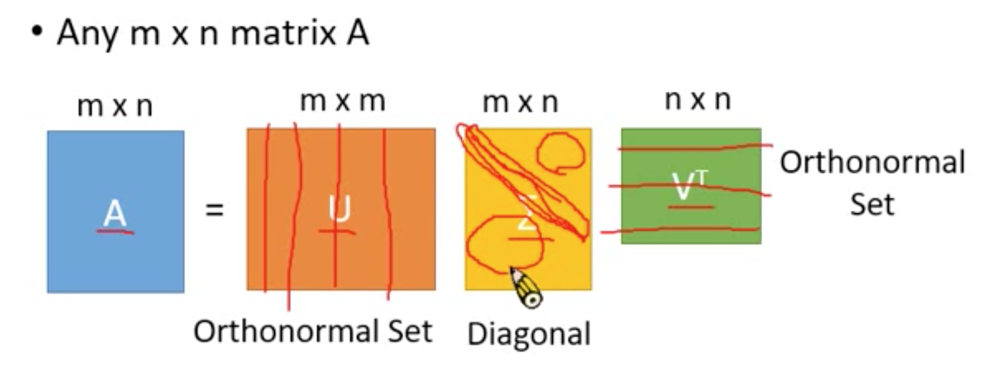
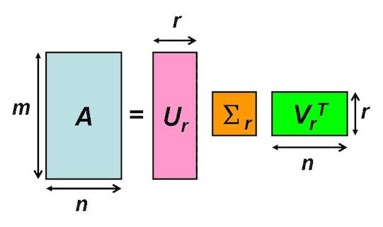
SVD 的概念就是，任一一個矩陣 \(A_{m \times n}\)，它都可以拆解成三個矩陣（\(U_{m \times n}, \Sigma_{m \times n}, V^T_{n \times n}\)）的相乘。

其中，\(U_{m \times n}\) 的 columns 是 Orthonormal，而 \(V^T_{n \times n}\) 的 rows 是 Orthonormal，\(\Sigma_{m \times n}\) 是 Diagonal(只有對角線有非負的值，且由大到小)。

(在線性代數中，一個內積空間的正交基（orthogonal basis）是元素兩兩正交的基。稱基中的元素為基向量。 假若，一個正交基的基向量的模長都是單位長度1，則稱這正交基為標準正交基或”規範正交基”（Orthonormal basis）。)

• \(\Sigma_{m \times n}\) 會是一個長得像這樣的矩陣，且 \(\sigma_1 \ge \sigma_1 \ge \ldots \ge \sigma_k\)

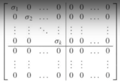
而 \(\sigma_r, ~~where~~1 \le r \le k\) 是奇異值（singular value），而 r 越小也代表了該值越重要，換句話說，含有越多訊息，因此我們可以只保留 \(\Sigma\) 較重要的前面幾行得到一個相似的矩陣 \(A\)。用較小的儲存空間就可以得到接近原始的矩陣 \(A\)。

\[A_{m \times n} \approx U_{m \times r} \times \Sigma_{r \times r} \times V^T_{r \times n}\]

參考線代啟示錄-奇異值分解 (SVD)的圖，

回到我們的 word-embedding。我們可以利用 SVD 進行去噪及降維，刪除一些不那麼重要的訊息，用來解決 Co-occurrence matrix 稀疏性的問題。

我們也不需要再將相乘矩陣，直接使用 𝑼 就好，每一列就代表一個 target word。

• Each row of the (truncated) matrix 𝑼 is a k-dimensional vector that represents the ‘most important’ information about a word.
• A practical problem is that computing the singular value decomposition for large matrices is expensive.

這邊看一個例子，

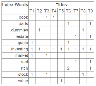
下圖是一個 Co-occurrence matrix \(~A_{m \times n}\)

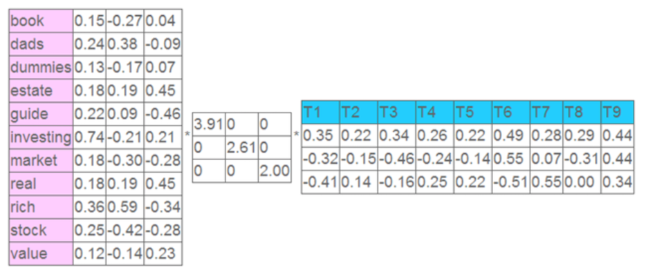
將上面的矩陣 \(A\) 使用 SVD 分解、降維，只留下前三個特徵值。每個特徵值的大小表示對應位置的屬性值的重要性大小，左奇異矩陣的每一列即代表每個詞的特徵向量，右奇異矩陣的每一行表示每個文件的特徵向量。

取每個向量後兩維的對應值投影到一個二維空間，如下所示

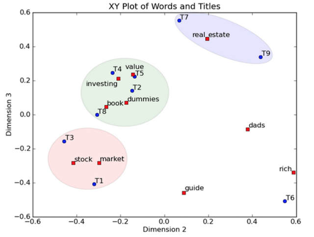
上圖中，一個紅色的點對應一個詞，一個藍色的點對應一個文件。當這些點被投影到空間中，我們可以對這些詞和文件進行分類，比如說stock和market可以放在一類，real和estate可以放在一類，按這樣的分類結果，我們就可以知道文件中哪些事相近的詞，所以當使用者利用詞搜尋文件的時候，我們就可以利用相近的詞（在向量空間中相近的詞、被歸為同一類的詞）進行檢索，而不是只是使用完全相同的詞搜尋。

---

Matrix factorization - Positive Pointwise mutual information(PPMI)

Pointwise mutual information(PMI)

• Raw counts favour pairs that involve very common contexts.
  E.g. the cat, a cat will receive higher weight than cute cat, small cat.

• We want a measure that favours contexts in which the target word occurs more often than other words.

• A suitable measure is pointwise mutual information (PMI):

\[PMI(x, y) = log \frac{P(x, y)}{P(x) \times P(y)}\]

簡單來說，我們可以用 PMI 公式來看兩個字之間的關係。

現在我們把 \(x\) 看成我們的 target word，\(y\) 看成我們的 context word，

• We want to use PMI to measure the associative strength between a word \(w\) and a context \(c\) in a data set \(D\):

\[PMI(w, c) = log \frac{P(w, c)}{P(w) \times P(c)} = log \frac{\#(w, c)/|D|}{\#(w)/|D| \cdot \#(c)/|D|} = log \frac{\#(w,c) \cdot |D|}{\#(w) \cdot \#(c)}\]

但根據上面的公式，會發現一個問題，PMI is infinitely small for unseen word–context pairs, and undefined for unseen target words. (如果 \(w\) 和 \(c\) 並沒有共同出現過，再取 log，整個值會變成 -Inf)

所以這時候就有了 Positive Pointwise mutual information(PPMI)。

• In positive pointwise mutual information (PPMI), all negative and undefined values are replaced by zero:

\[􏰜􏰜􏰝􏰞􏰍􏰂􏰠PPMI(w, c) = max(PMI(w, c), 0)\]

• PPMI assigns high values to rare events, it is advisable to apply a count threshold or smooth the probabilities.

看一個例子，

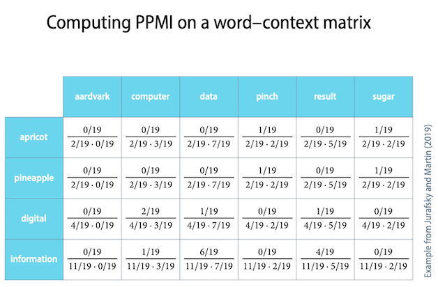
下圖是一個 Co-occurrence matrix，列是 target words，行是 context words

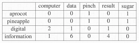
假設這篇文章總共只有 19 個字，這裡我們計算 x = information，y = data 的 PMI 值，

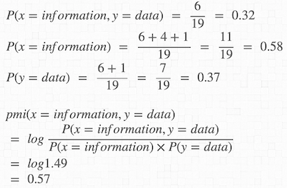
根據同樣的方式可以求出所有 target words 對應的 context words 的 PMI 值。

---

Language models

• A probabilistic language model is a probability distribution over sequences of words in some language.
• Recent years have seen the rise of neural language models, which are based on distributed representations of words.
• By the chain rule, the probability of a sequence of 𝑁 words can be computed using conditional probabilities as

\[p(w_1, w_2,\ldots, w_N) = \prod_{k=1}^N P(w_k|w_1 \ldots w_{k-1})\]

• To make probability estimates more robust, we can approximate the full history \(w_1 \ldots w_N\) by the last few words (馬可夫鍊):

\[p(w_1, w_2,\ldots, w_N) = \prod_{k=1}^N P(w_k|w_{k-n+1} \ldots w_{k-1})\]

---

Language models - N-gram models

• An n-gram is a contiguous sequence of n words or characters.
  E.g. unigram (Text), bigram (Text Mining), trigram (Text Mining course)

• An n-gram model is a language model defined on n-grams – 
a probability distribution over sequences of n words.

• n-gram 是一種語言機率模型。一句話出現的機率是一個聯合模型。如果一個詞的出現只考慮前面一個字，那就是 bi-gram；如果一個詞的出現考慮前面兩個字，那就是 tri-gram。

Formal definition of an n-gram model

• \(n\): the model’s order (1 = unigram, 2 = bigram, …)
• \(V\): a set of possible words (character); the vocabulary
• \(P(w\mid u)\): a probability that specifies how likely it is to observe the word \(w\) after the context
  (n − 1)-gram \(u\)

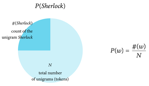
Unigram model

n = 1 不考慮前面出現的字。

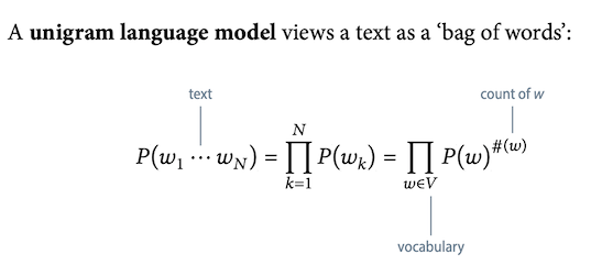
Thus contexts are empty.

MLE of unigram probabilities

---

Bigram models

n = 2 考慮前面出現的一個字。

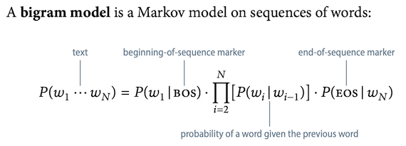
Thus contexts are unigrams.

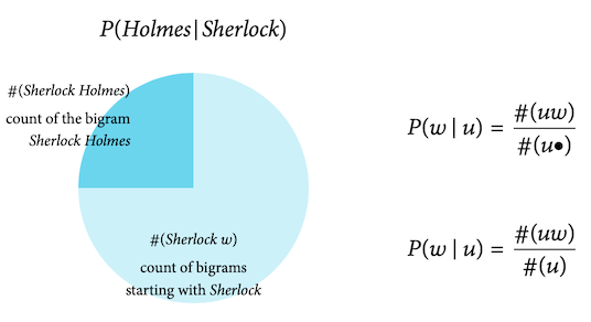
Estimating bigram probabilities

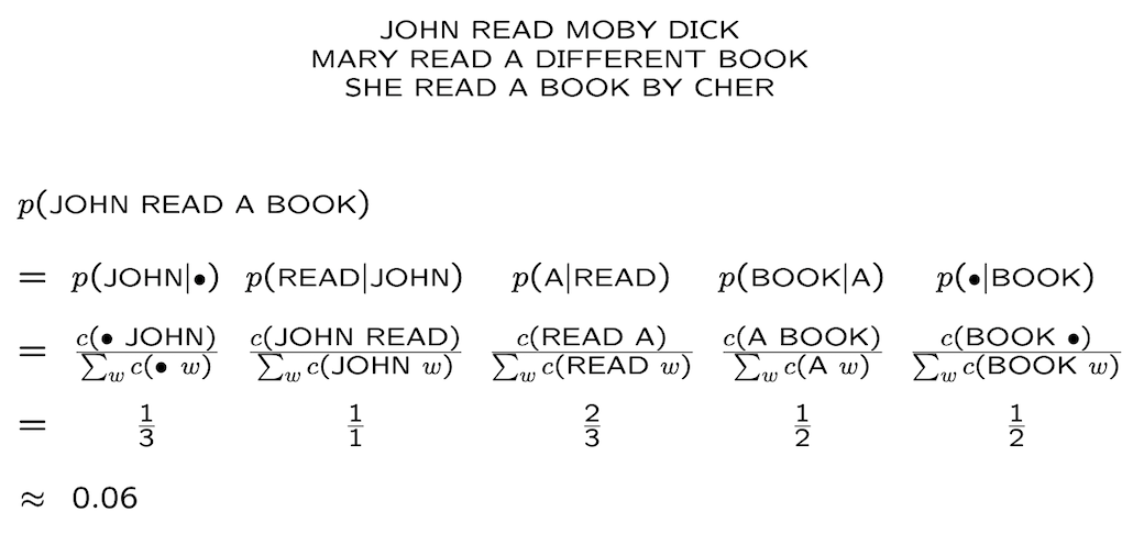
Example (source)

---

Smoothing

當在計算 bigram 時可能會碰到兩個字完全沒有相鄰的狀況，這會導致算出來的機率等於 0。（如下圖）

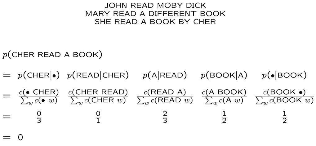
這種時候就需要用到，smoothing。

Smoothing methods

• Additive smoothing
• Good-Turing estimate
• Jelinek-Mercer smoothing (interpolation)
• Katz smoothing (backoff)
• Witten-Bell smoothing
• Absolute discounting
• Kneser-Ney smoothing

上面的狀況碰到的是，”CHER” 後面沒有出現 “READ” 的狀況，而導致機率等於0，但如果現在是 “CHER” 這個字從未出現在資料集中呢？這種狀況時，smoothing 便派不上用場了。

• In addition to unseen words, a new text may even contain unknown words. For these, smoothing will not help.

Unknown words
建立一個 token ，如果是 unknown words 就用 當作普通的單詞處理。

• A simple way to deal with this is to introduce a special word type UNK, and to smooth it like any other word type in the vocabulary.
• When we compute the probability of a document, then we first replace every unknown word with UNK.

---

Language models - Neural networks as language models

Advantages of neural language models

• Neural models can achieve better perplexity than probabilistic models, and scale to much larger values of n.
• Words in different positions share parameters, making them share statistical strength. (Everything must pass through the hidden layer.)
• The network can learn that in some contexts, only parts of the 
n-gram are informative. (implicit smoothing, helps with unknown words)

word2vec

• word2vec 是 word embedding 的一種

• word2Vec 主要有 CBOW (continuous bag-of-words) 和 skip-gram 兩種模型

• CBOW 是給定上下文，來預測輸入的字詞；Skip-gram 則是給定輸入字詞後，來預測上下文

---

Reference:
732A92 Texting Mining
詞向量介紹
自然語言處理 – Vector Space of Semantics
[NLP] 秒懂词向量Word2vec的本质
李宏毅老師的線性代數 - SVD
NLP 笔记 - 再谈词向量
機器學習筆記之二十二——PCA與SVD
線代啟示錄-奇異值分解 (SVD)
自然語言處理 – Pointwise Mutual Information
NLP Lunch Tutorial: Smoothing
機器學習五分鐘：自然語言處理（NLP）的N-gram模型是什麼？
詞向量(one-hot/SVD/NNLM/Word2Vec/GloVe)