


[Text Mining]Text classification
This post is based on the 732A92 Texting Mining course, given by Marco Kuhlmann at LiU in 2019.
Text classification
- Text classification is the task of categorising text documents into predefined classes.
Evaluation of text classifiers
最簡單的檢視預測結果好壞的方法就是將 predict 出來的類別與真實的類別做比較。(預測必須要在 test data,換句話說之前並沒有參與任何 training 的過程。這點在做所有 Machine Learning 的方法都很重要,在做 model 測試前不要碰 test data。)
Accuracy
The accuracy of a classifier is the proportion of documents for which the classifier predicts the gold-standard class:
\[\textrm{accuarcy} = \frac{\textrm{number of correctly classified documents}}{\textrm{number of all documents}}\]Accuracy and imbalanced data sets
上面的 accuracy 看起來非常合理啊,去計算分類正確的比例來判斷這個分類器是否預測準確。但,如果其實資料本身的類別並不平均呢?
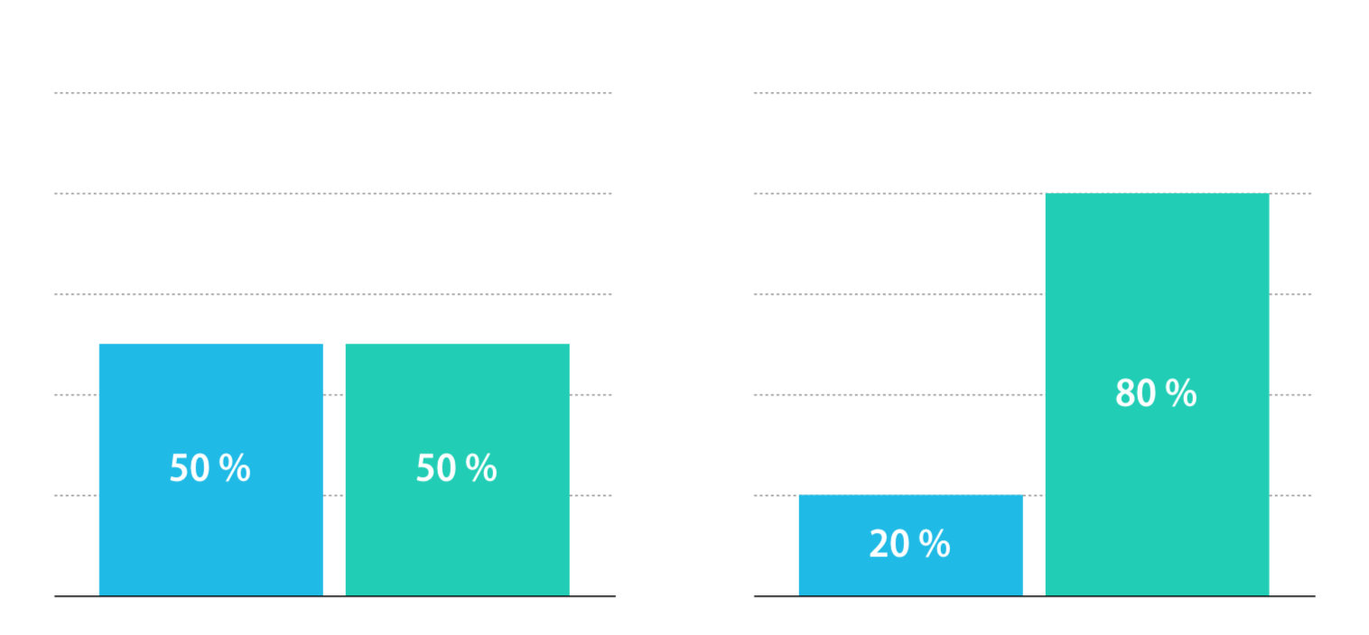
根據上圖,我們只要把所有資料都猜綠色的 class,這樣 accuracy 就能有 80%。從這個例子可以知道,
-
Evaluation measures are no absolute measures of performance. 如果今天得到 accuracy 是 80% 我們並無法確定這樣的準確率的好壞,要根據每個問題去判斷。
-
Instead, we should ask for a classifier’s performance relative to other classifiers, or other points of comparison. E.g.’Logistic Regression has a higher accuracy than Naive Bayes.’
-
When other classifiers are not available, a simple baseline is to always predict the most frequent class in the training data.
Precision and recall
-
Precision and recall ‘zoom in’ on how good a system is at identifying documents of a specific class.
-
Precision is the proportion of correctly classified documents among all documents for which the system predicts class.
- Recall is the proportion of correctly classified documents among all documents with gold-standard class.
F1-measure
A good classifier should balance between precision and recall.
\[\textrm{F1} = \frac{2 \cdot \textrm{precision} \cdot \textrm{recall}}{\textrm{precision + recall}}\]Naive Bayes classifier
Bayes’ theorem
We know that \(C\) is classes, \(x_i, i = 1, \cdots,n\) is features. Using Bayes’ theorem, the conditional probability can be decomposed as
\[p(C|x_1,..., x_n) = \frac{p(C)~p(x_1, \cdots,x_n|C)}{p(x_1, \cdots,x_n)}\]也就是,
\[\textrm{posterior} = \frac{\textrm{prior} \times \textrm{likelihood}}{\textrm{evidence}}\]根據上式,我們可以將分母視為常數,因為 features \(x_i, i = 1, \cdots,n\) 的值是給定的,且與 \(C\) 無關,所以可以得到
\[\begin{align} p(C, x_1, \cdots,x_n) & = p(C)~p(x_1,\cdots,x_n|C) \\ & \propto p(C)~p(x_1|C)~p(x_2,\cdots,x_n|C,x_1) \\ & \propto p(C)~p(x_1|C)~p(x_2|C, x_1)~p(x_3,\cdots,x_n|C,x_1,x_2) \\ & \propto p(C)~p(x_1|C)~p(x_2|C, x_1)~p(x_3|C, x_1, x_2)~p(x_4,\cdots,x_n|C,x_1,x_2,x_3) \\ & \propto \cdots\\ & \propto p(C)~p(x_1|C)~p(x_2|C, x_1)~p(x_3|C, x_1, x_2) \cdots p(x_n|C,x_1,x_2,\cdots ,x_n) \\ \end{align}\]Naive Bayes assumption
Naive Bayes 假設 \(p(x_i|C, x_j) = p(x_i|C), \textrm{for} ~ i \ne j\)
根據 Naive Bayes 的假設,前面的式子我們可以寫成,
\[\begin{align} p(C|x_1,..., x_n) & \propto p(C, x_1, \cdots,x_n) \\ & \propto p(C)~p(x_1|C)~p(x_2|C)~p(x_3|C) \cdots p(x_n|C) \\ & \propto p(C)~\prod_{i=1}^n p(x_i|C) \end{align}\]根據上面的推導過程,我們可以得到,
\[p(C|x_1,..., x_n) = \frac{1}{Z}~p(C)~\prod_{i=1}^n p(x_i|C)\]Naive Bayes classifer
而 Naive Bayes classifer 就是取各個分類 \(C_m, m = 1, \cdots, k\) 中 \(p(C|x_1,..., x_n)\) 值最大的為最後的分類結果。換句話說,我們可用這樣的式子表示
\[C_m = \mathop{\arg\max}_C p(C|x_1,..., x_n) = \mathop{\arg\max}_C p(C)~\prod_{i=1}^n p(x_i|C)\]而 \(C_m\) 就是最後的分類結果。
Two Classic Naive Bayes Variants for Text
- Multinomial Naive Bayes
- Data follows a multinomial distribution (多項分布)
- Each feature values is a count (word occurrence counts, TF-IDF weighting, …)
- Bernoulli Naive Bayes
- Data follows a multivariate Bernoulli distribution
- Each feature is binary (word is present / absent)
Reference:
732A92 Texting Mining
如何辨別機器學習模型的好壞?秒懂Confusion Matrix
wikipeida - 單純貝氏分類器