Decision Tree

Decision Tree是什麼？

簡單來說，decision tree 是一個分類模型。

• Tree-based methods partition the feature space into a set of rectangles, and then fit a simple model (like a constant) in each one.

這是 Pattern Recognition and Machine Learning 裡頭的定義。

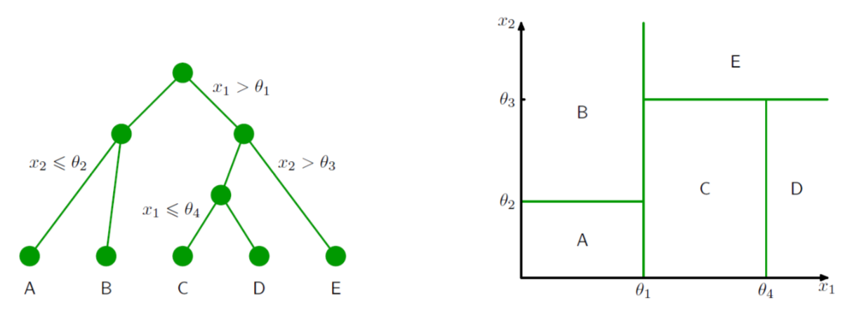
根據上圖，想像一下，在右邊的二維座標平面上有一堆散布的點，而 decision tree，就是將這個平面一一分割，每一個框框都是一個分類結果。但我們可以用右邊那樣一層一層的樹枝結構狀來表示右邊難懂的圖。（這裡的例子是二維平面，當變數 \(x_i\) 增加時，這樣的概念可以推廣到多維空間）

每一個分支都像是一個 if-else 問題，如果是就選某一邊，不是就選另外一邊。

上圖左，我們可以看到有兩個變數，\(x_1\), \(x_2\)，第一關是 \(x_1 > \theta_1 \)，如果小於就往左邊分，如果大於就往右邊分，以此類推往下繼續細分，最後給予分類結果。最後共分成 A, B, C, D, E 五個類別，也就是右邊的五個框框。

Decision Tree 又可以分為

1. Regression trees - 最後分類結果為連續變數

2. Classification trees - 最後分類結果為類別變數

名詞

• Root node (The Root) - 第一個起始的點
• (Internal) Nodes - 中間的節點。上方會有箭頭指向 node，且 node 也會往下指向其他點。
• Leaves (terminal nodes) - 最後的節點，也就是最後的分類結果。

如何分類？

假如今天我有一份 data，decision tree 是如何決定要先使用哪一個變數與什麼值作為分割呢？

分割的原則是，這樣的分割要能得到最大的資訊增益 (Information gain, IG) ([資料分析&機器學習] 第3.5講 : 決策樹(Decision Tree)以及隨機森林)

資訊量根據最後的分類結果可以使用，

1. Regression trees:
   • MSE (mean-squared error)
2. Classification trees:
   • Entropy (Deviance)
   • Gini impurity
   • Missclassification error

在 Classification tree 裡，Entropy 和 Gini impurity 是常用的兩種方式， 詳細的公式請參考 Wikipedia

假如今天碰到兩種 model 算出來的資訊量都ㄧ樣，請選擇比較簡單的那個 model。（分支、leaves node 較少）

R 範例 這裡使用 tree 這個 library 做範例，另外還有像是 rpart 也是做 decision 常用的 package。

library(tree)
data("iris")

# 使用 Entropy (Deviance)
fit <- tree(Species ~ Sepal.Length + Petal.Length, iris, split = c("deviance"))
plot(fit)
text(fit, pretty=0)

summary(fit)


# 使用 Gini impurity
fit <- tree(Species ~ Sepal.Length + Petal.Length, iris, split = c("gini"))
plot(fit)
text(fit, pretty=0)

summary(fit)

優缺點

• 優點：
  1. Simple to understand and interpret. 容易理解與解釋
  2. Able to handle both numerical and categorical data. 可以用在類別與 numerical 資料
• 缺點
  1. Low bias and high variance with respect to the training data. （當 decision tree model 變得太過複雜時，太多 nodes，就會導致 overfitting (bias-variance trade off 的狀況）

所以為了讓 model 不要 overfitting，我們可以使用 pruning 的方式，砍掉底下的樹枝。

在 R 可以使用，prune.tree()，並且可以使用 best 這個參數來決定最後要保留多少 leaves。

使用剛剛最後的 fit示範

prune_fit <- prune.tree(fit, best = 5)
plot(prune_fit)
text(prune_fit, pretty=0)
summary(prune_fit)

這時候 leaves 由原本的 9，修剪到了剩下 5，但 Misclassification error rate 卻是相同的。修剪過後的 model 較簡單，且 variance 也會比較小，在預測上表現也會較佳。

Reference:
[資料分析&機器學習] 第3.5講 : 決策樹(Decision Tree)以及隨機森林
StatQuest: Decision Trees
The Elements of Statistical Learning
Pattern Recognition and Machine Learning